In developing using virtual machines or containers it doesn’t take long before you’ll need to interact with a bridge network. They’re extremely common as a base networking configuration when working with multiple VMs on a single host, but learning about bridge networks can get confusing quickly, and even moreso when interacting with other network features like VLANs. This post is intended to be the start of an overview of bridges and why they’re useful when developing with virtual machines.

What are bridges?

Before we talk about what a “bridge network” is, we need to talk about what a “bridge” is. In the early days of ethernet, clients connected on the same Local Area Network (LAN) were connected to the same physical wires, typically a single coaxial cable. Clients would use Medium Access Control (MAC) protocols to ensure that they were not talking at the same time and interfering with eachother’s packets. One major problem with this is as you scale the number of clients, your throughput goes down significantly due to increasing likelihood of collisions.

Engineers at Digital Equipment Corp in the 1980s came up with a way to help improve this reduction in performance, by splitting each LAN into separate sections that shared a single wire, also called a “collision domain”. In between each collision domain would be a store-and-forward switch, which would be responsible for forwarding packets from one domain to their destination domain, but blocking packets if they were already on their destination domain. This effectively reduced the number of clients competing for access to the same medium, increasing throughput. The store-and-forward switches became known as bridges.

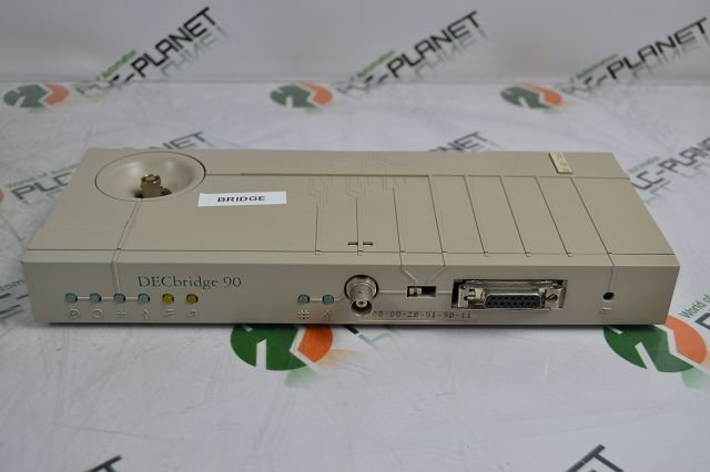
An early ethernet bridge. The front coax connector goes to one LAN (called the backbone) and the top coax connector goes to the other (called the work group).

The layer in the OSI model that deals with MAC is the datalink layer (layer 2), so this is why it’s common to hear that bridges are layer 2 devices that join networks.

How do they work?

During operation it is the responsibility of the bridge to maintain a forwarding information base to determine whether and how to forward packets that it receives. It typically does this with Contend-Addressable Memory (CAM) tables, which are a hardware implemented associative array that allow for quickly determining if a address is present in memory. The CAM table is populated as packets arrive with the source address and interface, and forwarded to the interface stored for the destination address. If the destination address is not stored in the CAM table, the packet is “flooded” across all interfaces. This is called “Unicast Flooding”, and is the basis for how all modern switches work.

One interesting problem that quickly arises from the unicast flooding technique is that many networks have loops in them. In cases of loops and no mitigating techniques, packets flooded to all interfaces will loop back to the same bridge device again and again, bringing the network to a halt.

Layer 3 protocols like Internet Protocol (IP) keep track of “hop counts” as the packet passes through the network, allowing packets which exceed a prescribed time-to-live (TTL) to be dropped, which mitigates this issue. Layer 2 protocols were not built with this luxury. Instead, they rely primarily on the Spanning Tree Protocol (STP) to ensure that bridges are only connected in ways that avoid loops, and any links that would create a loop are dropped. Other techniques to avoid network failures due to flooding are techniques like Shortest Path Bridging and TRILL.

Bridges vs Switches

Switches are a modern evolution of bridge technology, with several important performance improvements. Notably, instead of using software to define a CAM table for forwarding, switches will use custom ASICs to maintain forwarding information. Switches also will typically have more than 3 or more ports, where a conventional bridge may only have two.

Bridge Networks

In the context of virtual machines a bridge network is one that creates a software defined bridge and allows virtual hosts to be added to it, as you would plug a machine into the port of a physical switch. A bridge network can be configured to be completely isolated from the outside network, or connected to the network via the physical network interface.

The most basic tools to create an modify bridges come from the iproute2 toolkit, which includes the ip utilities as well as the bridge utility. To create a new bridge called br0:

# ip link add name br0 type bridge

This creates a new bridge device called br0 that other physical and virtual interfaces can be connected to. The typical way to connect a physical port to the bridge is by configuring the master/slave parameters on the interface, in this case enp3s0:

# ip link set enp3s0 master br0

Note that by setting the physical interface as a slave of the bridge, the bridge device is now the one that is associated with an IP address. To connect a virtual machine to the bridge, the attachment is typically done in Linux by a virtualization library such as libvirt.

Note that the software defined bridge operates just as a physical bridge does, including storing forwarding information. This information can be displayed via the bridge utility, and might look something like this:

# bridge fdb show
62:fa:c3:85:4e:e6 dev enp3s0 vlan 1 master br0
08:e6:89:c1:18:84 dev enp3s0 vlan 1 master br0
5a:5d:60:9c:1c:89 dev enp3s0 vlan 1 master br0
...

This output is indicating that the bridge br0 learned that MAC 62:fa:c3:85:4e:e6 is associated with device enp3s0 (our physical interface).

To Be Continued…

In part 2, we will discuss VLANs and how they interact with virtual bridges.